A Competition Model of Menu Cost

The Model

The model will feature the following three properties:

1. Asymmetric
   The cost to decrease prices is a small constant while the cost to increase prices is positive and increasing in the size of price adjustment.

2. Quadratic or exponential right tail
   When the firm increases prices, the initial menu costs are low, but the costs will increase quadratically or exponentially as it wishes to increase another unit of prices. (The same setup as in Rotemberg (1982))

3. Responsive to current market inflation and inflation expectations
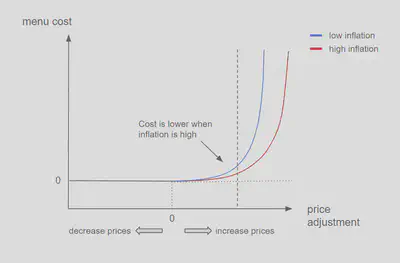
   The menu cost curve is responsive to inflation and inflation expectations. When inflation and inflation expectations are low, the right tail curve are steeper (i.e. more costs associated with one unit of price increase)

Here’s the menu cost curve visualized: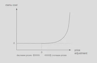

To explain why these three properties make sense, let’s consider a grocery store that can set prices independently and let’s consider a setup of oligopoly where there are a few other similar grocery stores in the same place. Consumers exhibit “lock-in” effects (i.e. they are partially “locked into” purchasing from a particular store once they have begun purchasing from it).

First of all, I would like to clarify that the menu cost here should not be taken at face value–it is not the technological barrier to change prices (like replacing the physical menus and printing new price tags and catalogs) that is the main source of menu costs¹. But rather we are considering the costs (or the fear) of potentially losing locked-in consumers when they increase the prices higher than their competitors².

Therefore, the first property comes naturally. There is almost no cost to lower prices, but the costs to increase prices will be high.

As the store increases the prices of goods, there is a margin that the consumers will not be conscious of. Maybe Safeway sells a dozen coke a few dollars more expensive than in Target, but most consumers won’t notice and churn. However, there must be an upper limit. When the consumers realize that Safeway is selling it much more expensive than Target, they will not continue to do their shopping at Safeway. Therefore, the initial cost of increasing prices is low, but the costs will grow faster than linear. This is the second property.

The third property decrees that the upward price change costs are larger when inflation and inflation expectation is lower. This is the most important property. High inflation (or inflation expectation) in the economy has two implications: a) the competing firms are also subject to higher costs and more likely to increase prices, b) the consumers will be more “forgiving” when they see a price increase. Therefore, since the store will have less “worry” of losing customers when they decide to increase prices in the period of high inflation, the associated cost will be lower.

How is it a better flavor of nominal rigidity?

1. Persistent Price Shocks
2. Inflation Spiral

We can consider this in two phases.

In phase 1, there are some initial price shocks that lead to an increase to the cost of the firms (e.g. raw materials, oil prices, upstream supply). The current inflation rate is low, and therefore the competition menu cost is relatively high, and the firms are less willing to increase prices.

But as the supply-side shock persists for a while, some firms will eventually need to increase their prices so that they are not selling below their costs. Again, even though at this time, the competition menu cost is high, they still need to increase their prices.

Now we begin phase 2. As some firms start to increase their prices, the overall inflation rate in the market starts to increase. When the inflation rate is higher, the competition menu cost declines. This results in more firms starting to increase their prices–they don’t have any fear of losing customers since the overall inflation is higher and their competitors are also increasing prices. Therefore, we can see a Domino effect that could drive the economy into an inflation spiral. However, a real inflation spiral (i.e. firms increasing their prices non-stop) is quite hard, since the competition menu costs are exponential.

This can generate persistent price shocks and offer an explanation for the inflation spiral.

Empirical examination

There are several empirical examinations that we could do to determine if this proposition is in line with reality or not.

1. Regional oligopolies: naturally, if a certain city offers fewer choices of grocery shopping (an extreme example: only one supermarket exists in the radius of 100 miles), then it faces less competition. We can test if the prices in these places are more flexible than other regions where competition is more tangible.

2. Speed of inflation: as implied by our two phase hypothesis, the inflation rate would start to increase slowly, then faster.